
An Artificial Neural Network (ANN) is a series of algorithms that endeavors to recognize underlying relationships in a set of data through a process that mimics the way the human brain operates[1]. Neuron typically has a weight that adjusts as learning proceeds. This article focuses on the basic mathematical and computation process in the ANN.
Artificial Neuron
An artificial neuron is a mathematical function that models biological neurons. A Neuron can receive input from other neurons. The neuron inputs are weighted with and summed () them before being passed through into an activation function. Figure 1 shows the structure of an artificial neuron.

ANN is a supervised learning that its operation involves a dataset. The dataset is labeled and split into two part at least, namely training and testing. We have expected output (from the label) for each input. During the training process, the parameter weights and biases are updated in order to achieve a result that is close to the labeled data. To identify model performance, we evaluate the model to the testing dataset to verify how good the trained model is. To get more detail how ANN learn, let begin with the last two neurons connection.

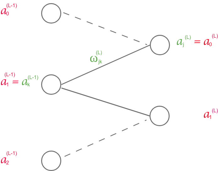
is a neuron with an activation
is an index of layer. It is not an exponential.
In the training phase, the sample data is fed through the ANN. The outcome of the ANN is inspected and compared to the expected result (the label). The difference between the outcome and expected result is called Cost/Error/Loss. There are several cost functions can be used to evaluate the cost in analyzing model performance. One of the common ones is the quadratic cost function.
The cost for the network in Figure 2 in form of quadratic cost function is:
The total cost of a feed through the ANN are:
Equation (1) and (2) show that the closer the outcome of ANN to the expected result, the smaller the cost will be. The cost can be thought as a mathematical function of weights and biases . Hence, the fittest model can be achieved by minimizing the cost to find the suitable weights and biases.
Gradient Decent
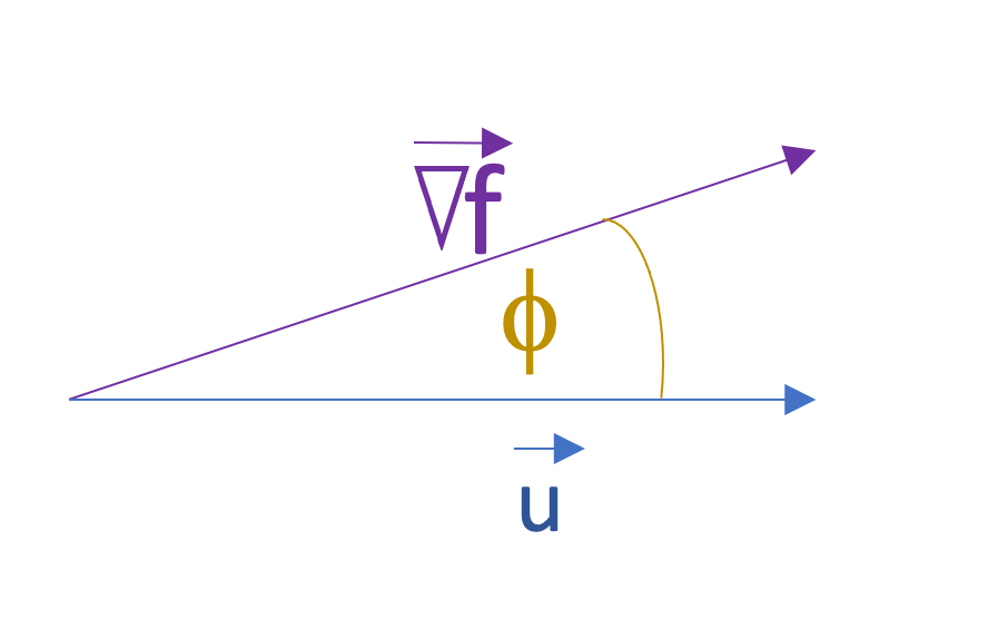
In multivariable calculus, gradient of a function presented as . Gradient of a function in the direction of vector in Figure 3 expressed as:
If is a unit vector, the . Thus, the Equation (3) can be written as
The maximum result of Equation (4) gained at . Since the is a unit vector, it can be evaluated from as
The minimum slope / steepest descent is gained at the opposite of the steepest ascent (at )
Since ANN is essentially minimizing the cost function, the gradient descent is used as basic idea to find the best fit ANN parameters (weights and biases) in the learning process.
The same method also implemented to get bias update.
is a learning rate. It is an additional value added how much the gradient vector we use to change the current value of weights and biases to the new ones. If is too small, adjustment of weight will slow. The convergency to local minimum will longer. However, if it is too high, the search of local minimum might be oscillated or reach overshoot. Ilustration of gradient descent in 3 dimention plot ilustrated in the Figure 4. Of course it is hard to plot the gradient descent that cover all weights of the ANN.
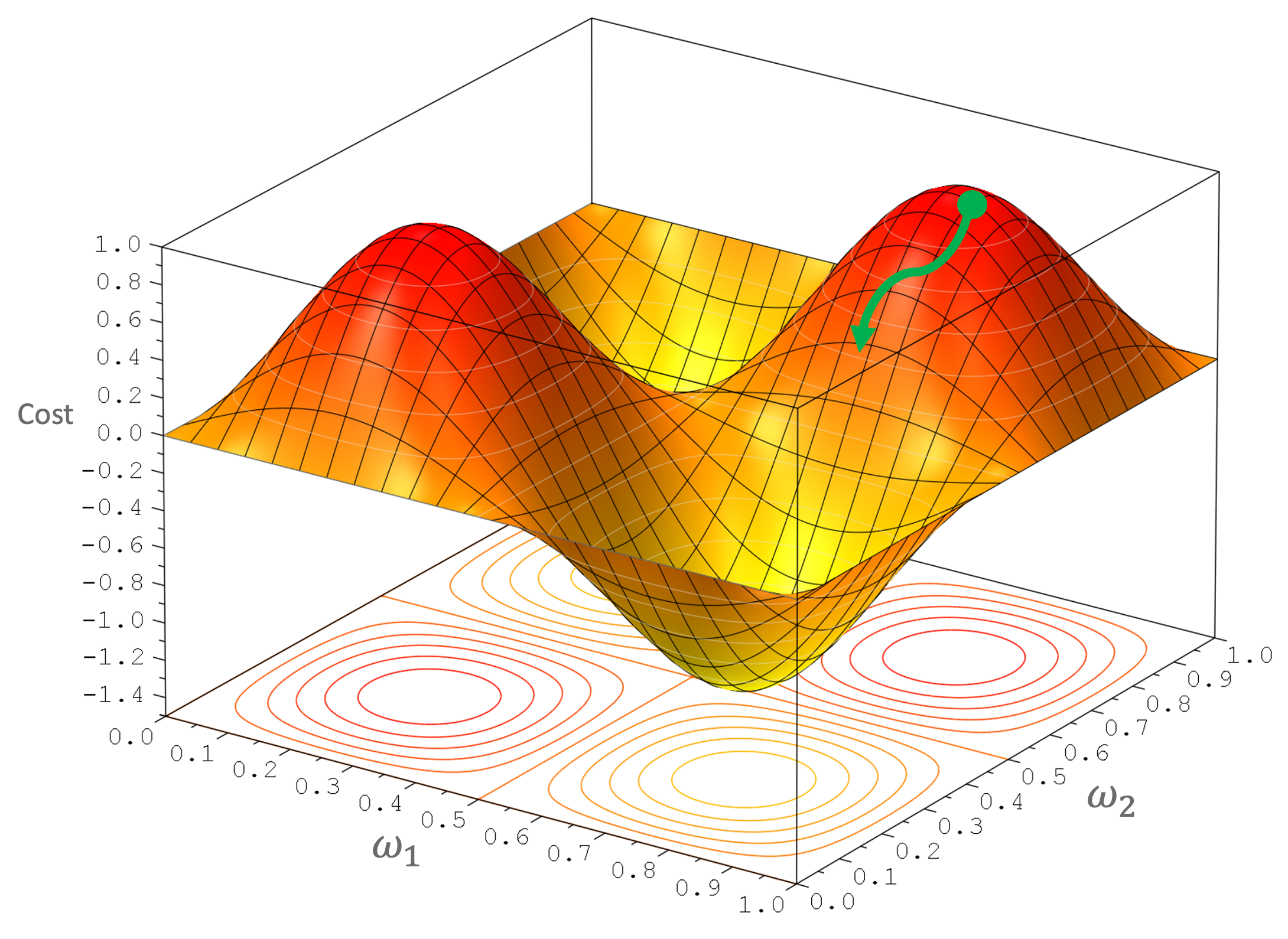
Iterative training will let the cost function gradient move in the direction of green line to the local minimum as ilustrated in Figure 4. In fact, gaining global minimum is the ideal condition. However it is very difficult since we start the movement from a random location (random weight at initial training). Reaching local minimum is acceptable in finding the optimal model. If we want a better model, we can retrain the ANN by generating new random or setting different initial values of weights and biases.
Mathematical Notion
Previously has been discussed that the basic idea to find the optimal model is the gradient of a multivariable function. The topic of the gradient in calculus cannot be separated from the discussion of function theory and derivative. Since an ANN can have several layers, the chaining function and chaining derivative are needed in analyzing its mathematical notion. The 3Blue1Brown team has a good illustration in describing chain function and derivative in ANN graphically. This article adopts the illustration in describing the chaining rule.
By using the neuron topology in Figure 1, we can identify that:
Let define to simplify mathematical expression.
Thus,
Correlation between variables described graphically as:
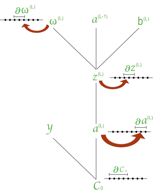
The graphical correlation can be extended to the previous neuron.
The sensitivity of cost function to the change of weight is expressed as:
From Equation (1) and (10)
The coeficient of 2 indicates that deviation between and significantly gives impact to the
From Equation (9) and (10)
From Equation (8) and (10)
So mathematical expression in Equation (10) can be written as:
Since the cost can be thought as a function of weights and biases, the gradient of cost function of each training can be expressed in partial derivative of all weightes and biases. Thus we can present it as a vector matrix.
The sensitivity of cost function to weight can be extended to analyze sensitivity of cost function to bias.
From Equation (8):
Thus,
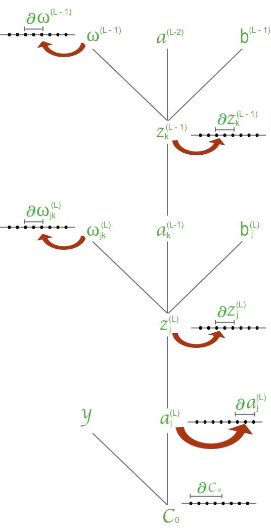
To get a more comprehensive neuron connection, Figure 7 denotes ANN with a more detailed subscript and superscript that show index neuron order and layer.
So that,
Figure 7 shows that impacts the value of and . Thus, the rate of changes to is evaluated as (sum over layer L):
Generally, Equation (11) can be written in a fully indexed notation as:
Component of Equation (15) can be evaluated using the same approach as Equation (14)
If the cost function defined as , then
Numerical Computation
To complement the explanation about neural networks, in this post we will use an example provided by Tobias Hill with a slight modification in notation to meet our notation convention in the previous chapter. The neural network structure showed in Figure 8.
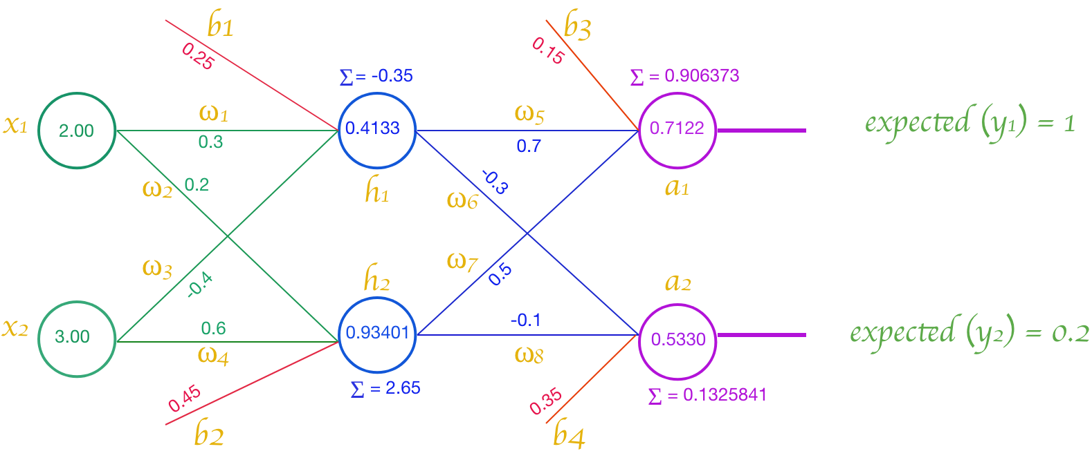
The activation function we use is sigmoid, and the learning rate of
The cost function of the ANN is evaluated with Equation (1).
Feed Forward
First of all, Let’s evaluate output of neuron by implmenting sigmoid activation fuction as showed in Equation (16).
The result and expected values of the ANN can expressed as matrix vector.
The total cost of first feed to the ANN is evaluated with Equation (2):
Equation (2) shows that is essentially a function of or
Back Propagation
Weight of
Thus,
By using the same method, we can evaluate the update the other weights and biases in the last layer.
To update bias, we use the similar way as updating weight.
Weight of